

Simulation of Voltage Source Inverter Induction Motor Drive
Background
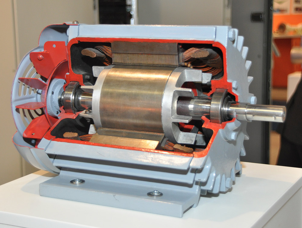
The induction machine is one of the oldest AC electro-mechanical power conversion devices [1]. In the late 19th century, engineers pioneered the first single-phase induction motor, followed soon by the three-phase variant. Compared with other popular motor types (e.g. DC or synchronous), the induction motor is typically lower cost and has higher reliability. This has pushed the technology to become the dominant player in industrial applications. See Fig. 1a for an example induction motor.
To fully realize the potential of the induction motor at various torque / speed operating points, it must be driven from a variable frequency power source. In the mid to late 20th century, a breakthrough in power electronics was made with the introduction of the transistor. This device enabled efficient, robust, high-frequency power converters to be created. The voltage source inverter (VSI) became the most prevalent foundation for today’s variable frequency drives used to control modern induction motors.
Voltage Source Inverter (VSI)
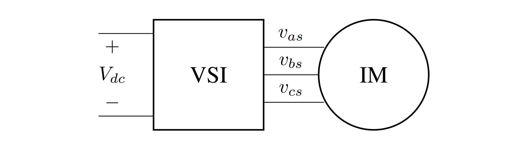
The voltage source inverter (VSI) is used to convert between DC and AC power. Fig. 1b shows a VSI connected to an induction machine. For normal motoring operation, power is drawn from the DC input power supply ($ V_{dc} $) and is modulated to AC power on the output phases ($v_{as}$, $v_{bs}$, and $v_{cs}$).
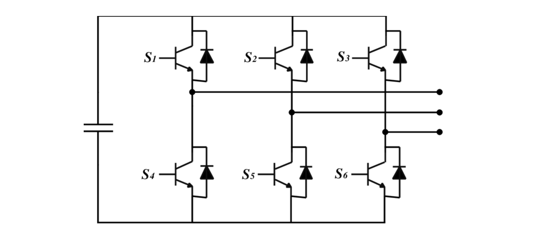
Internally, the VSI is composed of several components. To provide a stiff voltage source, a DC link capacitor is connected across the DC input. Three half-bridges are connected across the DC link capacitor. Each half-bridge is composed of two power electronic switches. The mid-point of each half-bridge becomes the phase connection for the induction motor. See Fig. 1c for a schematic representation.
Recent Technology Advancements
The typical power electronic switch that is used in the VSI is either the insulated gate bipolar transistor (IGBT) or the metal-oxide semiconductor field effect transistor (MOSFET). MOSFETs are usually used for high frequency applications with lower voltage requirements, while IGBTs tend to be used for lower frequency, higher power applications. In recent years, two new promising switch technologies have been introduced: gallium-nitride (GaN) and silicon-carbide (SiC) [2]. These devices enable power converters to switch at higher frequencies while maintaining lower switching losses. When the VSI drives the induction motor using higher switching frequencies, the output voltage better approximates the reference and leads to lower current ripple due to the machine inductance acting as a filter. This reduces the losses in the induction motor and reduces torque ripple.
Motivation
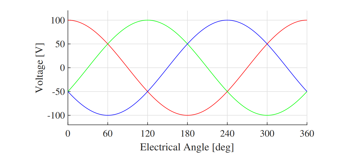
To create steady-state torque which rotates an induction motor, it can be shown that a three-phase balanced set of sinusoidal voltages must be applied to the motor phases, as shown in Fig. 2. These voltages can be expressed as the following, where $V_o$ is the amplitude of the voltage and $\omega_e$ is the electrical frequency.
Alternatively, these voltages can be represented in the complex $dq$ plane where the signals are given as: .
Modulation Techniques
The goal of the VSI is to reproduce the waveforms shown in Fig. 2 as accurately as possible. However, because the inverter uses switched-mode operation, only eight discrete voltage states are available at the phase terminals. Typically, duty cycle techniques are employed to create a time averaging effect. On average, the VSI replicates the desired reference waveforms, but at any instance in time, the waveforms are comprised of the eight discrete voltage states.
Six-Step Excitation
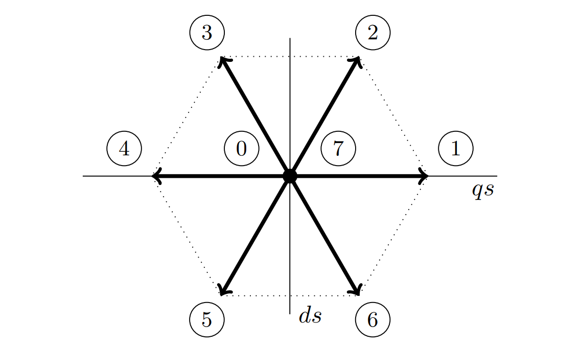
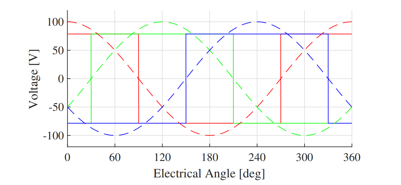
The most simple technique for driving an induction motor using the VSI involves direct use of the six active voltage vectors (1-6) to approximate the reference waveforms. Fig. 3a shows all possible VSI voltage vectors on the complex $dq$ plane. The six-step modulation technique applies each of the active voltage vectors for a portion of time. If each is applied for a $60^\circ$ segment, the fundamental component of the voltage waveform will equal the desired reference waveforms. Fig. 3b shows both the actual phase voltages and the fundamental component for six-step excitation. While simple, six-step operation creates large harmonics in the induction motor current, thus creating torque ripple. Alternative modulation techniques are preferred due to better harmonic properties.
Sine-Triangle Modulation
The sine-triangle modulation approach is shown in Fig. 4 for a single desired reference voltage (e.g. $v_{as}$). To implement this modulation, a high frequency triangle wave, referred to as the carrier wave, is required. The desired voltage reference is scaled by the DC bus voltage and compared to the triangle carrier. The output of this comparison is used for the gating signals to each half-bridge in the VSI.
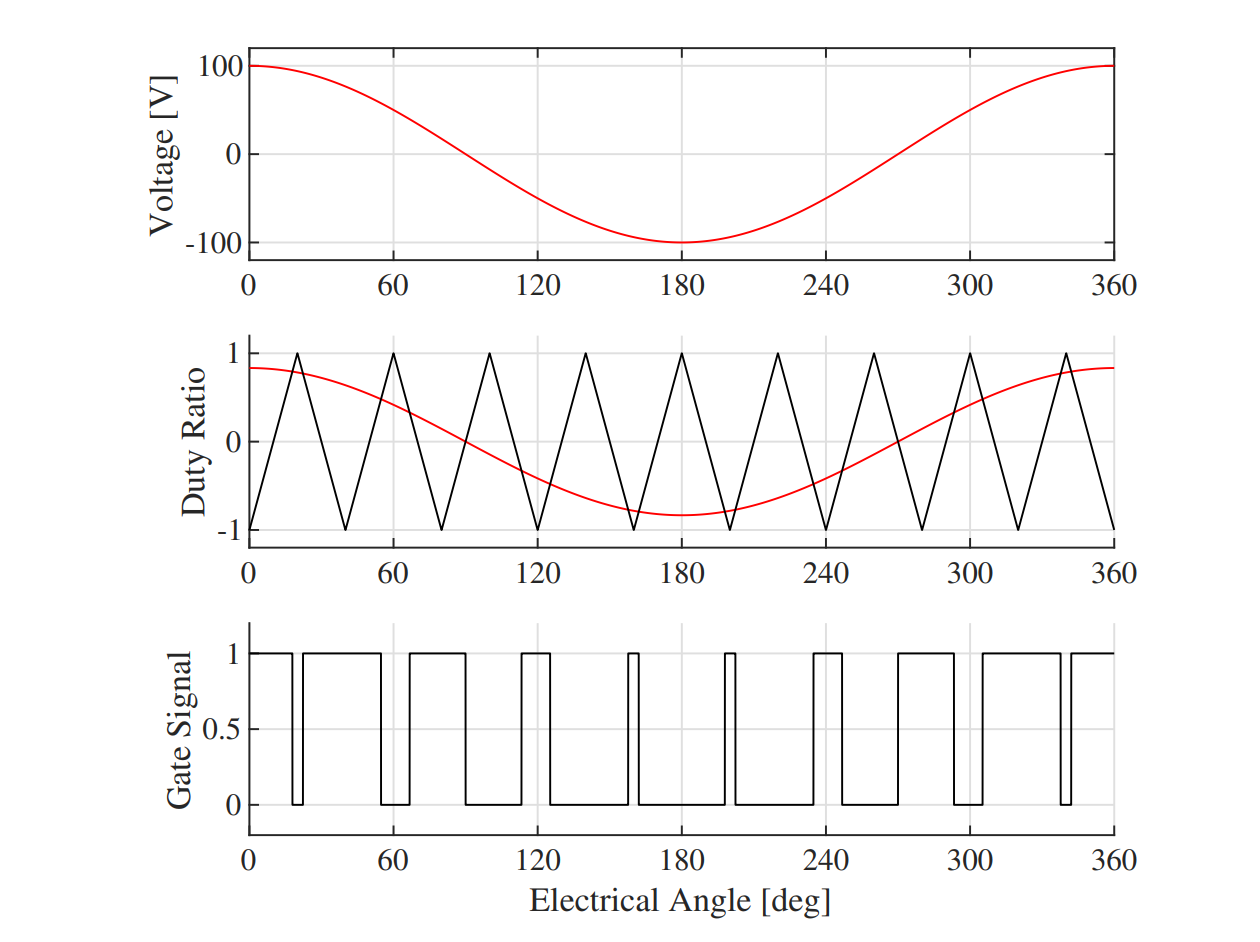
The advantages of the sine-triangle modulation technique include the ability to generate arbitrary reference waveforms using pulse-width modulation (PWM) and operating with a fixed switching frequency, but limit the induction motor phase voltage magnitude to $\frac{1}{2} V_{dc}$. This limitation occurs because the common-mode voltage on all three phases is fixed at half of $V_{dc}$.
Space Vector Modulation
The space vector modulation (SVM) algorithm can be related to both the six-step and sine-triangle modulation techniques. As extension to six-step operation, SVM adds the concept of duty cycle averaging to achieve average phase voltages which can arbitrarily lie on the complex $dq$ plane within the hexagon (see Fig. 3a), as opposed to the six fixed active voltage vectors [3]. SVM achieves this by mixing parts of the active voltage vectors (1-6) along with the zero states (0,7) within each switching interval.
Alternatively, SVM can be thought of as an extension to the standard sine-triangle modulation [4]. For this, a zero-sequence portion is added to each voltage command which depends on the instantaneous voltage references. To control the ratio of time spent in the two zero states (0,7), a parameter $0 \leq k_o \leq 1$ is defined. The final voltage reference is defined as $ v_{abc}^{**} = v_{abc}^* + v_{zs}^* $ where
$$ (1 - k_o) v^*_{min}] $$
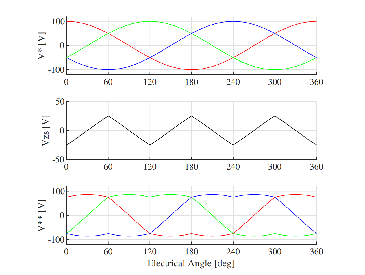
Fig. 5 shows the voltage references for the VSI when using SVM and generating the same voltage references as in Fig. 2. The zero-sequence component is shown in black. By adding this component to each phase voltage, the common-mode voltage does not appear on the induction motor, but acts to extend the usable DC bus voltage to about 15% more than with no zero-sequence injection.
Simulation
The induction machine can be modeled as a coupled set of non-linear differential equations. Typically, complex variables are used to represent the electrical quantities (encapsulating vector magnitude and phase information). When the mechanical system is included, the induction motor becomes a non-linear fifth order system.
The electrical quantities can be viewed from various reference frames, with common choices representing the stationary, rotor, or synchronous reference frames. The following equations model the stator and the rotor of the induction machine in the arbitrary reference frame, as well as the dynamics of the mechanical system. The coupling between the electrical and mechanical systems occurs due to the developed torque, which can be represented as the right hand side of the last equation. Together, these three equations model the entire induction machine dynamics.
$$ \frac{3}{2} \frac{P}{2} L_m \mathbb{I}m{ \bar{i}{qds}^s \bar{i}{qdr}^{s*}} $$
In the above equations, $r_s$ and $r_r$ are the stator and rotor resistances, $L_s = L_m + L_{ls}$ is the total stator inductance, $L_r = L_m + L_{lr}$ is the total rotor inductance, $L_m$ is the magnetizing inductance, $p = \frac{d}{dt}$ denotes the differentiation operator, $\omega$ is the arbitrary reference frame, $\omega_r$ is the rotor electrical speed, $\omega_m$ is the rotor mechanical speed, $P$ is the number of machine poles, and $J$ is the mechanical rotary inertia.
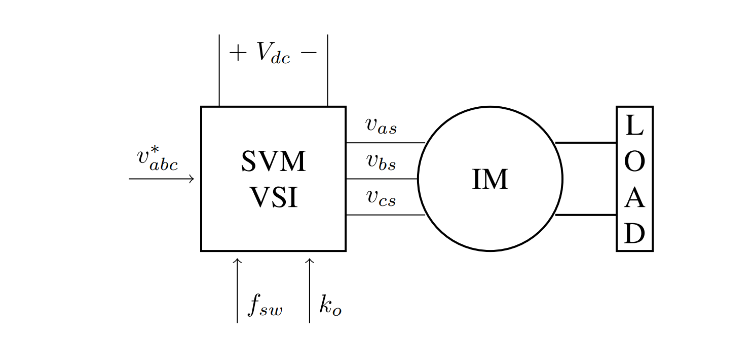
The choice of $\omega$ determines the reference frame; in this analysis, the synchronous frame is used such that $\omega = \omega_e$. For the simulation results that will be presented and discussed below, the following table summarizes the induction motor parameters. Fig. 6 shows the simulation block diagram that will be used. The inverter switching frequency $f_{sw}$ and zero state allocation scheme $k_o$ will be investigated.
| Parameter | Value | Units |
|---|---|---|
| $V_{rated}$ | 460 | $V_{rms,l-l}$ |
| $P_{rated}$ | 20 | hp |
| $f_{rated}$ | 60 | Hz |
| $P$ | 4 | poles |
| $Z_B$ | 14.20 | $\Omega$ |
| $V_B$ | 376 | $V_{pk}$ |
| $I_B$ | 26.5 | $A_{pk}$ |
| $T_B$ | 79.16 | N-m |
| $r_s = r_r$ | 0.355 | $\Omega$ |
| $x_{ls} = x_{lr}$ | 1.42 | $\Omega$ |
| $x_m$ | 34.1 | $\Omega$ |
| $M$ | 1.4 | sec |
| $s_{rated}$ | 0.03135 | – |
Baseline: Steady-State Operation
The first condition of interest is the baseline steady-state operation, where the induction machine falls into a stable operating point depending on the values of the resulting speed and torque. A constant load of 50% rated torque is applied. For this simulation, the inverter is operating at a fixed switching frequency of $f_{sw}$ = 3kHz at a DC voltage of 650V. Space vector modulation is used with the modulation index $M_i = 0.9$ and $k_o = 0.5$. Note that the ratio of the switching frequency to the fundamental is 50.
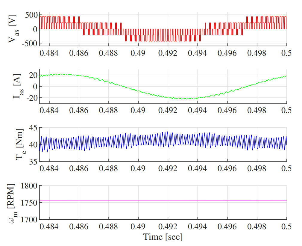
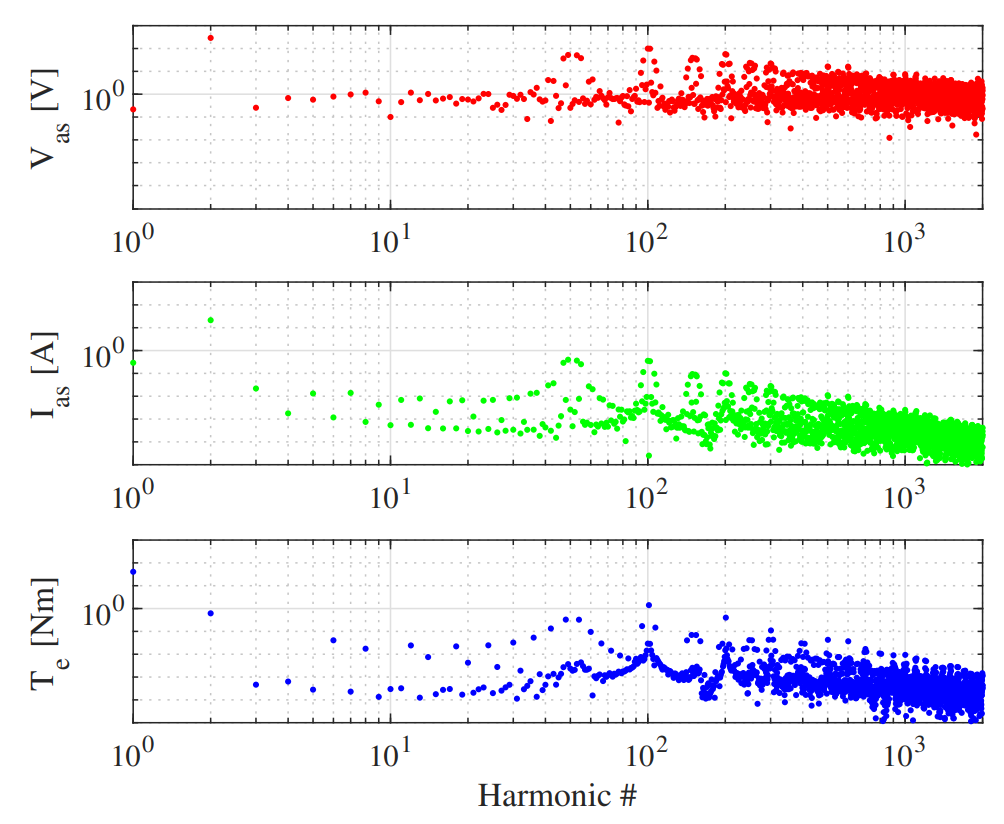
Fig. 7 shows the resulting waveforms from the simulation, with Fig. 7a showing the time domain waveforms and Fig. 7b showing the frequency content of the waveforms. In the time domain, the PWM nature of the applied phase voltage is obvious, but the resulting phase current is very smooth and sinusoidal due to the filtering effects of the motor inductance. The resulting torque has a DC component, but nearly 10% ripple. The resulting speed is approximately constant at 1755 RPM. To verify the steady-state simulation results, we can analyze the induction machine as its Thévenin equivalent circuit, where the equivalent complex impedance is given by
$$ \frac{x_m (x_{lr} + r_r/s)}{x_m + x_{lr} + r_r/s} $$
$$ Z_{th} = r_s + x_{ls} + \frac{x_m (x_{lr} + r_r/s)}{x_m + x_{lr} + r_r/s} $$
The critical or break frequency of an RL circuit is given by $f_c = R / (2 \pi L)$. Using $Z_{th}$ for the simulated induction machine, this results in $f_c$ = 101Hz. Because the phase voltage excitation PWM is at 3kHz, this is nearly 30x greater than the break frequency of the machine, so the nearly smooth current is reasonable.
Effects of VSI Switching Frequency
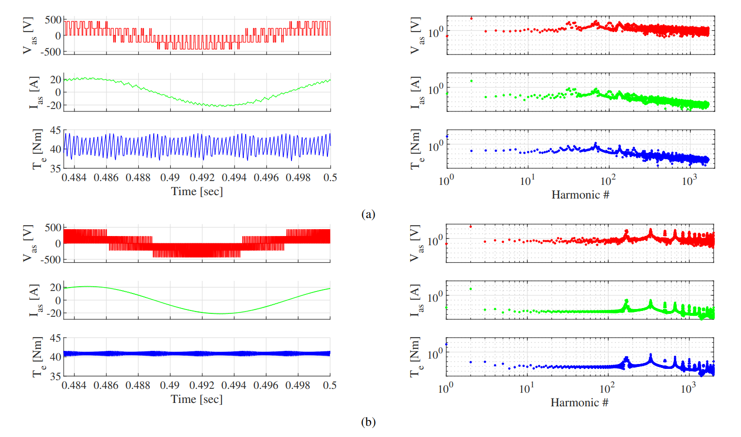
The switching frequency of the VSI plays a major role in the resulting ripple on the current and torque waveforms. Fig. 8 shows the simulated waveforms for different VSI switching frequencies. Fig. 8a and Fig. 8b show the resulting waveforms when $f_{sw}$ = 2kHz (20x machine break frequency) and $f_{sw}$ = 10kHz (100x machine break frequency), respectively. Notice that at large $f_{sw}$, the harmonic content of the waveforms is shifted to higher frequencies such that the signal energy near the fundamental is reduced. This results in cleaner current and torque time domain waveforms with less ripple. By increasing $f_{sw}$, harmonic losses in the induction motor are reduced, while inverter switching losses are increased. Full system applications must make an engineering trade-off between the machine and inverter losses.
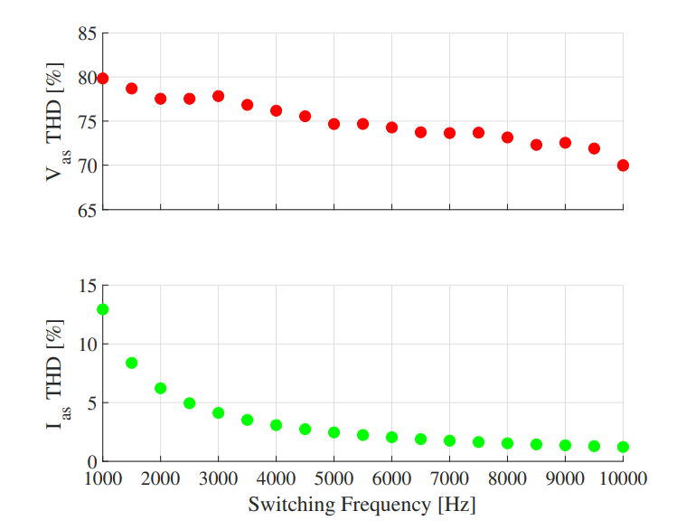
To characterize the improvement from increasing the switching frequency, various metrics can be analyzed. In this analysis, the phase current ripple is analyzed. The expected phase current is ideally sinusoidal, but due to the PWM VSI, current ripple increases as $f_{sw}$ decreases. The _total harmonic distortion_ (THD) of a sinusoidal waveform can be calculated as the following, where $x_1$ denotes the magnitude of the fundamental component, $x_2$ is the magnitude of the second harmonic, etc. This provides a metric for the amount of energy present in the waveform not at the fundamental frequency.
$$ \mathrm{THD} = \frac{\sqrt{x_2^2 + x_3^2 + x_4^2 + …}}{x_1} $$
To relate the VSI switching frequency to the THD of the phase voltage and current, multiple simulations were run for various $f_{sw}$. Fig. 9 shows the simulation results: when $f_{sw}$ = 1kHz (10x break frequency) and $f_{sw}$ = 10kHz (100x break frequency), the THD of the current waveform is 13% and 1.2%, respectively, showing an inverse logarithmic relationship between $f_{sw}$ and current THD. However, the voltage kept its high THD across $f_{sw}$.
Steady-State Operation With Various Constant Ko
The previous simulation results used a fixed value of $k_o = 0.5$. This partitions the zero voltage vector states evenly between vector 0 and 7 (see Fig. 3a for voltage vector definitions). By changing $k_o$, the ratio of the zero states is adjusted. This section of the analysis investigates the effects of setting $k_o$ to a constant value not equal to 0.5. A range of 0.2 to 0.8 is investigated. For example, when $k_o$ = 0.2, voltage vector 7 is used for 80% of the zero state, and the remaining 20% is spent in voltage vector 0. The theoretical time-averaged voltage in a single PWM cycle is the same, but it is achieved using different VSI switch combinations.
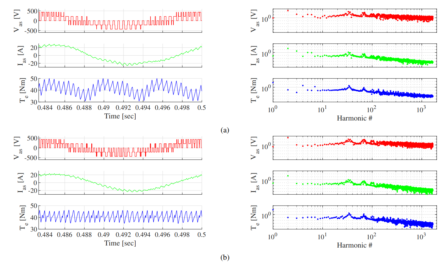
Fig. 10 shows simulation results for two values of $k_o$ = 0.2 and 0.35 ($f_{sw}$ = 2kHz). The current waveforms roughly match Fig. 8a, the equivalent scenario but with $k_o$ = 0.5. However, the torque waveform has much more ripple and harmonics than previously. When $k_o$ = 0.35, the torque waveform reduces its harmonics, but adds other high frequency content. The effects on the torque waveform occur due to the interactions between the three phase currents in the synchronous reference frame.
Furthermore, by setting $k_o \neq 0.5$, the frequency content of the waveforms is spread and shifted. In Fig. 10a, the frequencies between the fundamental and PWM carrier has significantly more energy than in Fig. 8a. By setting $k_o$ = 0.5, this spread of energy is reduced.
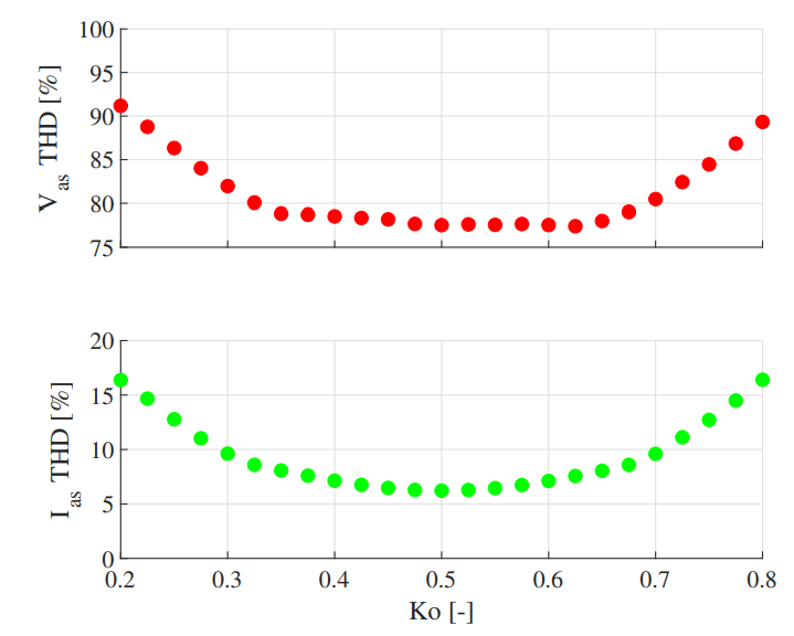
To further investigate the effects of $k_o$ on the induction motor drive, the full range of $k_o$ = 0.2 to 0.8 is simulated. The total harmonic distortion (THD) of the resulting voltage and current waveforms is calculated and presented in Fig. 11. At $k_o$ = 0.5, both the phase voltage and current have a minimum in THD. As $k_o$ is brought away from its nominal value of 0.5, the THD of both the voltage and current increases. This leads to the conclusion that, for fixed $k_o$, the least THD in voltage and current is achieved at $k_o$ = 0.5.
Steady-State Operation With Changing Ko
Per the previous section, the optimal constant $k_o$ value is 0.5; this reduces THD in both voltage and current waveforms to the minimum value. However, by dynamically changing $k_o$, a further reduction in THD is possible.
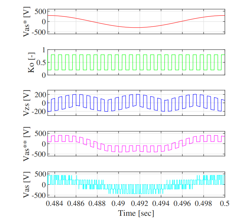
Fig. 12 presents the flow of signals inside the SVM VSI. The input voltage reference $v_{as}^*$ is summed with the zero-sequence voltage $v_{zs}^*$ (based off of the present $k_o$ value) to form the final voltage command $v_{as}^{**}$. This voltage reference is then modulated with the PWM triangle carrier to form the voltage applied to the induction motor $v_{as}$. Notice that the waveform for $k_o$ is not constant; each PWM cycle, it jumps between a minimum and maximum value for 50% of the time. If the minimum and maximum values for $k_o$ are both 0.5, this approach simplifies to the results from the previous section. However, by changing the min and max $k_o$ values, the harmonic performance is changed.
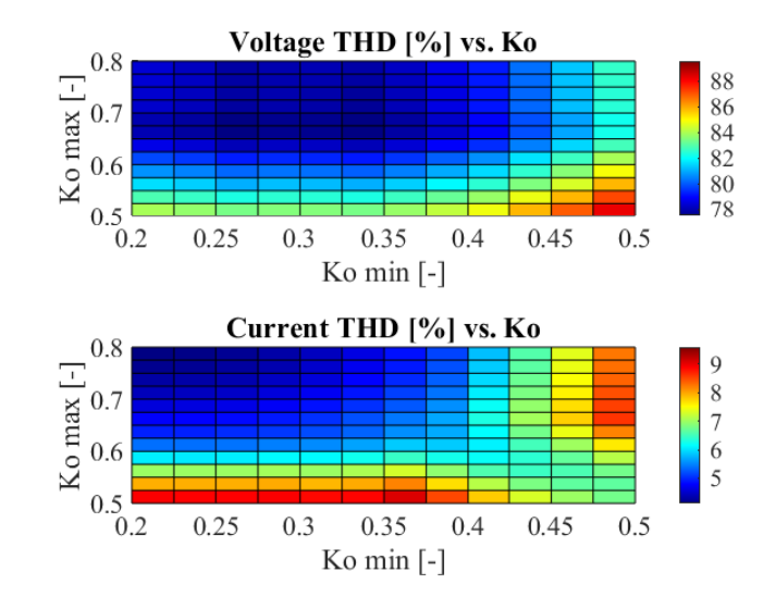
Fig. 13 shows the results of 169 simulations, one for each box in the map. In each simulation, $f_{sw}$ is held constant at 3kHz, but the min and max values for $k_o$ are changed. The THD is calculated for both the phase voltage and current, and expressed as a percent corresponding to a color. The previous section results for $k_o$ = 0.5 is found in the lower right-hand box, resulting in a current THD of about 7%. Following a line diagonal from the bottom right to the top left results in the THD values for when the min and max $k_o$ is symmetrical around the nominal 0.5 value, while off-diagonal boxes are asymmetrical. By alternating between symmetrical values of $k_o$, the THD of both the voltage and current waveforms is reduced. At $k_o$ = 0.2 and 0.8, the current THD is 61% of the nominal baseline ($k_o$ = 0.5).
Summary
This study analyzed the induction motor when driven by the voltage source inverter. Several modulation techniques were presented and related to each other. The space vector modulation technique was shown to have superior performance by extending the phase voltage range to 15% more than the sine-triangle modulation technique.
The induction motor was simulated using several configurations of the SVM VSI. Analysis of PWM switching frequency and zero voltage vector placement was performed. Results were compared in the time and frequency domain. Total harmonic distortion was used as the metric for evaluating the performance of the inverter configuration. It was found that higher switching frequencies result in less THD, along with dynamically changing zero voltage vector placements.
Future work may investigate changing the load of the induction motor and the dynamic effects of the modulation techniques. For example, using real-world drive sequences can help the application engineer determine optimal values for $f_{sw}$ and $k_o$ depending on system level requirements.
This analysis was performed during Spring 2020 for University of Wisconsin-Madison course ECE 711: Dynamics and Control of AC Drives.
References
-
B. G. Lamme, “The story of the induction motor,” Journal of the American Institute of Electrical Engineers, vol. 40, no. 3, pp. 203–223, March 1921.
-
J. Millan, P. Godignon, X. Perpina, A. Perez-Tomas, and J. Rebollo, “A survey of wide bandgap power semiconductor devices,” IEEE Transactions on Power Electronics, vol. 29, no. 5, pp. 2155–2163, 2014.
-
H. W. van der Broeck, H. . Skudelny, and G. V. Stanke, “Analysis and realization of a pulsewidth modulator based on voltage space vectors,” IEEE Transactions on Industry Applications, vol. 24, no. 1, pp. 142–150, 1988.
-
V. Blasko, “A hybrid pwm strategy combining modified space vector and triangle comparison methods,” in PESC Record. 27th Annual IEEE Power Electronics Specialists Conference, vol. 2, June 1996, pp. 1872–1878 vol.2.
New Post Notifications
If you read this far into this article, you might be interested in subscribing for email notifications about future new posts I write. I will never spam you! Every few months, I write a new article for this website, and will send you email about it. You can unsubscribe at any time. Thank you.